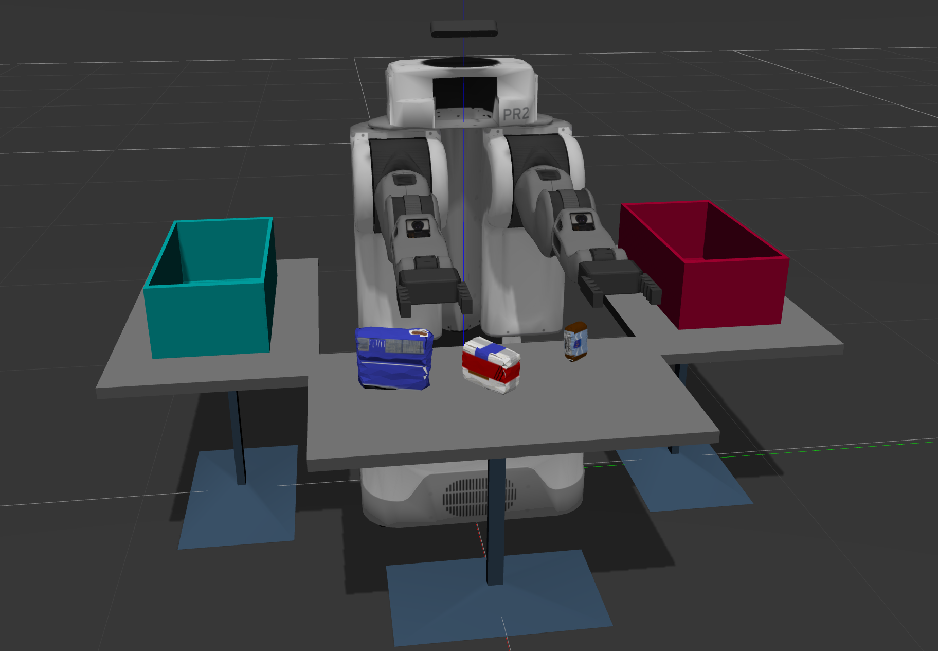
Perception pipeline for a PR2 robot using an RGB-D camera: filter raw point cloud data, segment objects, and classify them using a trained SVM model.
Filtering
Raw point cloud data goes through three filters before segmentation:
Statistical Outlier Removal — removes noise points whose mean neighbor distance falls outside a defined standard deviation threshold (k=20, stddev=0.1).
Voxel Grid Downsampling — reduces point density by averaging points within each voxel (leaf size 0.01m), keeping enough detail for recognition while reducing compute load.
Passthrough Filter — crops the scene to a region of interest along Y (-0.4 to 0.4) and Z (0.6 to 0.9) axes, focusing the robot on the tabletop.
RANSAC Plane Segmentation — separates the table surface (inliers) from objects (outliers) using a max distance of 0.01m.
Clustering
Used DBSCAN (Euclidean clustering) on a KD-tree representation of the point cloud. DBSCAN does not require a predefined number of clusters, making it well suited for unknown table arrangements.
Object Recognition
Each cluster’s color and surface normal histograms are extracted and matched against a trained SVM model (linear kernel, C=0.1). Training used 20–40 random poses per object per scene.
Object identification accuracy: 97%
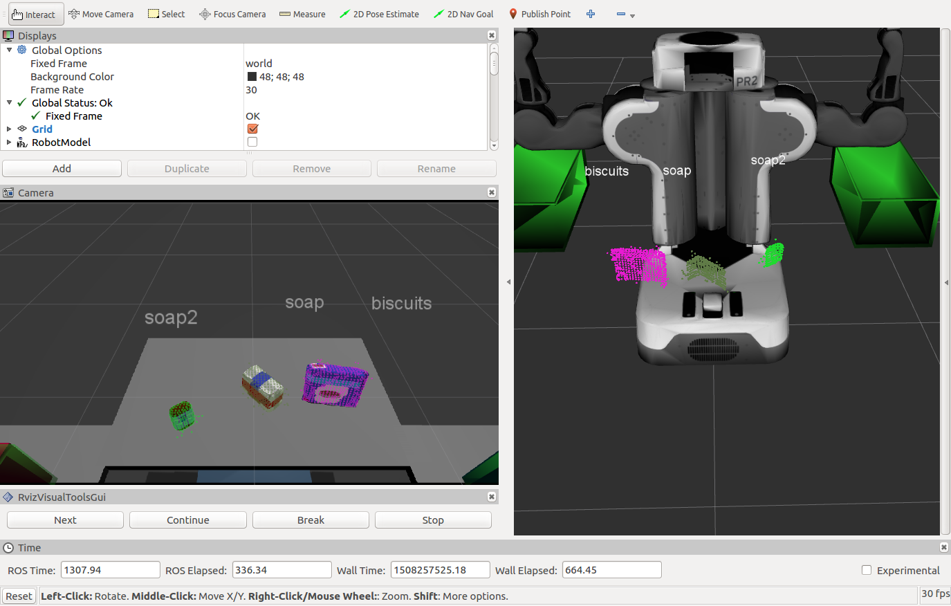
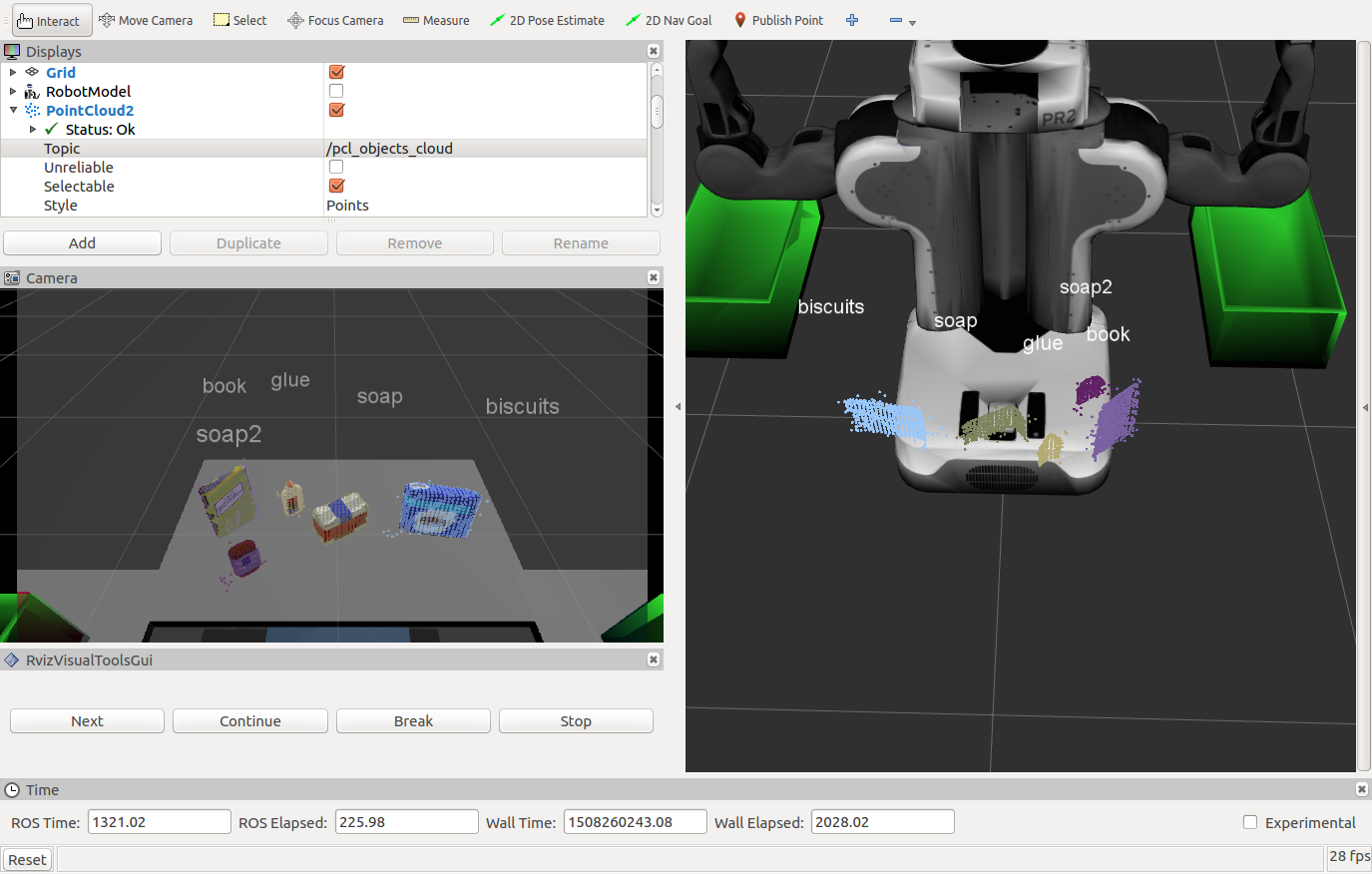
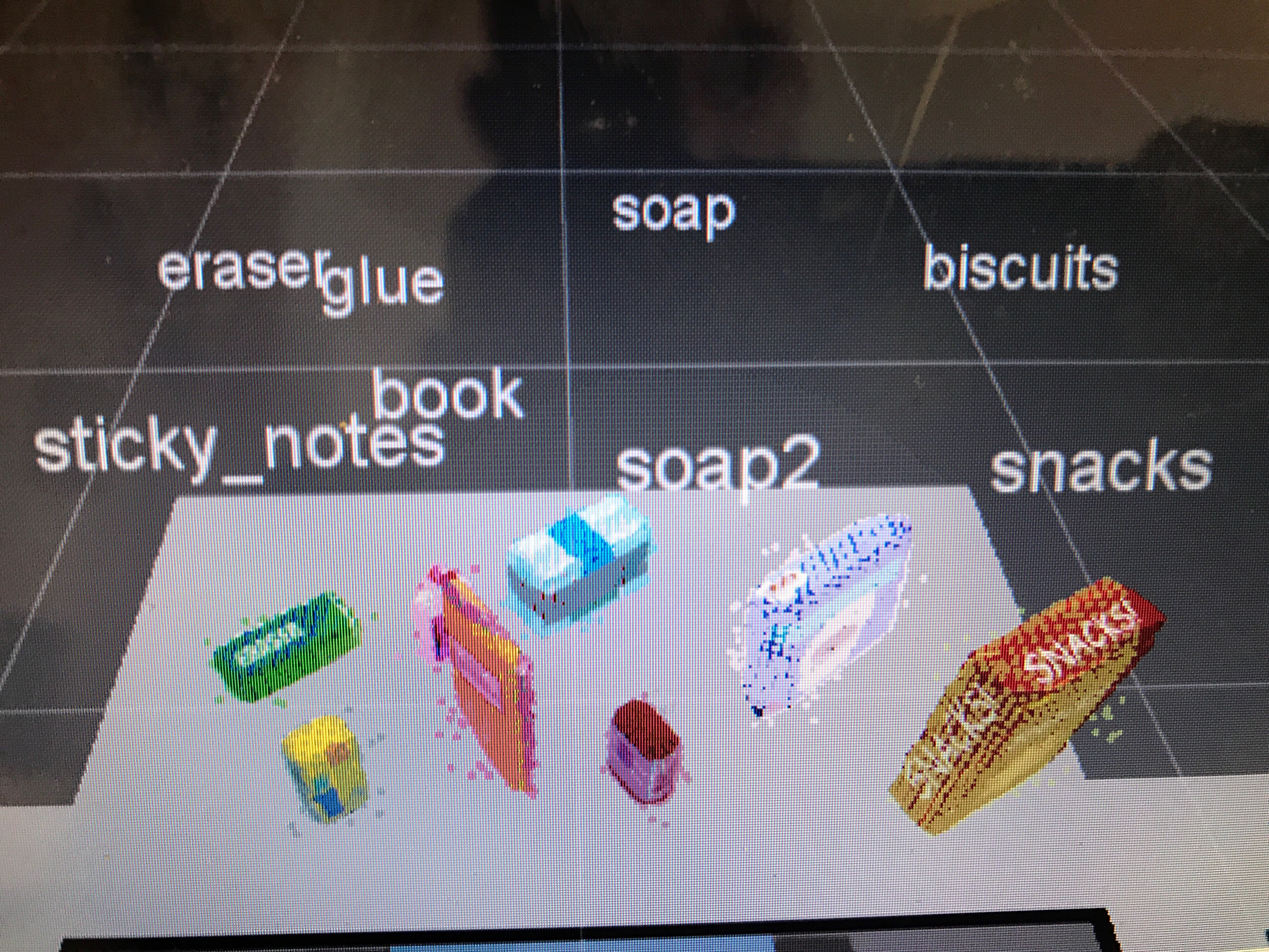
Test Scenes