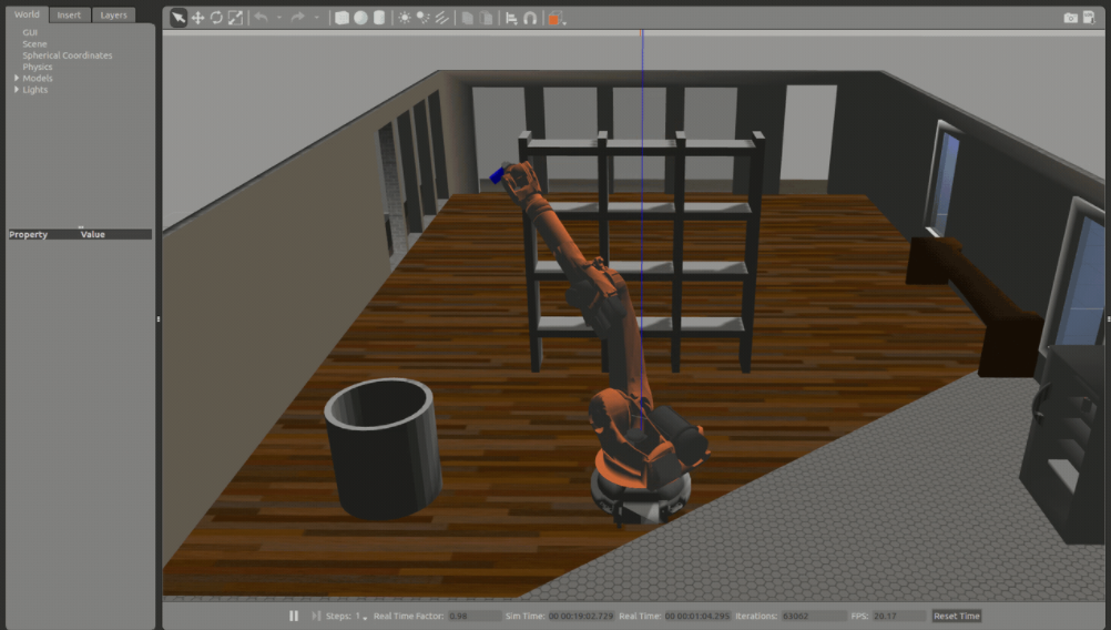
Programmed a Kuka KR210 6-DoF serial manipulator in Gazebo to pick a cylinder from a randomized shelf position and drop it into a bin.
Kinematic Analysis
Derived the DH parameter table from the KR210 URDF and built individual transformation matrices for each joint in Python using SymPy.
DH parameter reference frame:

| Links | alpha(i-1) | a(i-1) | d(i) | theta(i) |
|---|---|---|---|---|
| 0->1 | 0 | 0 | 0.75 | q1 |
| 1->2 | -pi/2 | 0.35 | 0 | -pi/2 + q2 |
| 2->3 | 0 | 1.25 | 0 | q3 |
| 3->4 | -pi/2 | 0 | 1.5 | q4 |
| 4->5 | pi/2 | 0 | 0 | q5 |
| 5->6 | -pi/2 | 0 | 0 | q6 |
| 6->EE | 0 | 0 | 0.303 | 0 |
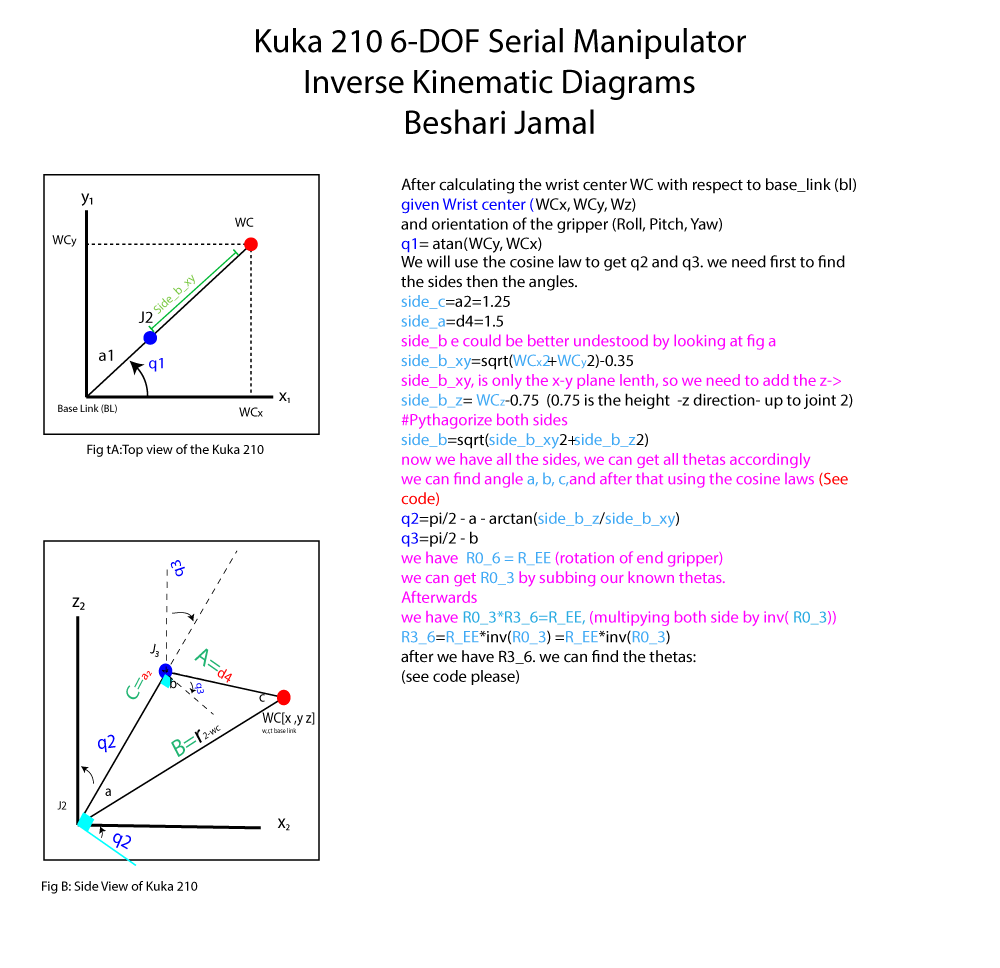
Inverse Kinematics
The KR210 has a spherical wrist (joints 4, 5, 6 intersect at joint 5), enabling a closed-form IK solution. The first three joints position the wrist center; the last three orient the end-effector.